Deriving the Sahm rule from the DIEM
The Sahm rule naturally arises in the Dynamic Information Equilibrium Model (DIEM) with noise
I realize that in the past I just kind of vaguely hinted that the Sahm rule was related to the “recession detection algorithm” threshold that’s based on the information equilibrium approach to economics. I thought I’d put a bit more meat on the bones of that argument. The Dynamic Information Equilibrium Model (DIEM) is a particular application of information equilibrium where you assume the process variables are exponential functions of time with different growth rates (see link to paper for more details). With regard the unemployment rate u, that means “equilibrium” should be defined in an ensemble of labor markets as an approximately constant log-linear decline:
Note that a similar observation was later made empirically in Hall and Kudlyak (2020)1.
Per the DIEM, these periods of equilibrium are interrupted by non-equilibrium shocks2, resulting in a pretty good description the structure of the unemployment rate that we see3:

We can see that the locations where the unemployment rate stops falling (i.e. “equilibrium” ends) are where recessions happen. Economist Claudia Sahm tried to use this information to work out a threshold that could be set to trigger automatic stabilizers. See for example, here:
The rule compares the average of the most recent three months of unemployment data to the minimum of the past year of those averages. If the most recent three months is more than 0.5 percentage points (pp) higher than the past year of three month averages, the rule indicates a recession is likely. It’s been honored with its own time series on FRED.
In a world without noise, the theoretical model (DIEM) would say the most recent data is the minimum due to that constant log-linear decline — therefore any increase in the unemployment rate means a non-equilibrium shock. However, when you have noise, you have to distinguish an increase just due to noise versus an increase due to a non-equilibrium shock. That runs us into a bit of detection theory.
If we do the transformations (minimum of previous 12 months of 3-month averages, 3-month average, compare to the threshold of 0.5 pp) to the theoretical model and the data, it looks like the following graph:

Let’s subtract the theoretical baseline calculated from the DIEM from the three month average and call this “Delta”. We obtain what looks a lot like a pure noise time series with a few spikes at the three major recessions prior to the pandemic:

That pure noise component is loosely normally distributed as we can see in a histogram vs Delta, while the spikes show up as a long tail to the right:

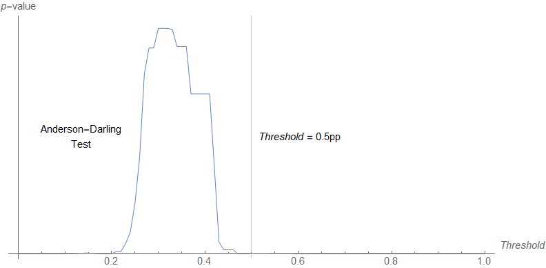
There are a lot of different ways to try to estimate that noise floor and separate out signals (e.g. a CFAR detector). A straightforward method is to set a threshold and test the remaining data (which is supposedly “noise”) for “normality” via a goodness of fit test. I used an Anderson-Darling test vs threshold value:
We can see that a value of 0.5 pp is a pretty safe choice for a deviation being outside the noise — above 0.5 pp, the p-value is infinitesimally small which tells us the resulting distribution is unlikely to be a normal distribution (i.e. it’s not noise).
Just looking at the deviation from the model, we can see that 0.5 pp is pretty far out in the tail:
The standard deviation of the model error for the 3-month averages is ~ 0.14 pp which means that 0.5 pp is ~ 3.6 standard deviations (3.6 σ). With monthly data, we’d expect to see a 3 σ event once every 30 or so years and a 3.5 σ event once every 180 years. This is getting into physics-levels of significance4, so that threshold should work pretty well.
The theoretical model (constant log-linear decline) plus the estimate of the noise in the data allows us to set a threshold for the detection of the leading edge of a rise of unemployment — the Sahm rule. You could of course create better estimates of the noise and its distribution5. However, the argument above is sufficient to show something like the Sahm rule would indicate the onset of a non-equilibrium shock. And that is its purpose — to provide a warning signal sufficient to enact automatic stabilizers.
With a value of (d/dt) log u ~ −0.1/year.
Modeled as a series of logistic functions in my 2018 paper.
The pandemic showed that the unemployment rate itself is the wrong measure — the actual measure should be closer to U3 minus layoffs (‘core’ unemployment). During the pandemic, layoffs were disconnected from the unemployment rate in a way that had not been seen in the post-war data. However, this is not critical to the discussion of the Sahm rule as it just caused the non-equilibrium shock to rise and fall faster than had previously been observed — it has not had an impact on the detection of future recessionary shocks as far as we can tell.
A standard heuristic for discoveries is 5 σ in particle physics whereas between 3 σ and 5 σ are “hints”; below 3 σ is usually nothing.
There is quantization noise of 0.1 pp, so the noise is not exactly normally distributed — it’d be better modeled as a convolution of a uniform distribution with a normal distribution. And per the theory, the noise is actually normally distributed in logarithm (the basis of the recession detection algorithm).


