The equity premium puzzle

Addressing the problem in the information equilibrium framework

Let me say up front this is not a solution to the equity premium puzzle, but rather showing how you might address it in the information equilibrium framework. Let’s start with the AD-AS model from this post

¹

:

\(\displaystyle \Pi \equiv \frac{d\langle AD\rangle}{dAS} = \langle n \rangle \frac{\langle AD\rangle}{AS}\)

I changed up a couple of symbols here because I’m going to introduce a second model for equities in a minute. Here Π is the price level, and ⟨n⟩ is the ensemble average of the individual market information transfer indices. What you should have in your head is a kind of “statistical equilibrium” picture where there are a distribution of information transfer indices nᵢ for each individual market producing output ADᵢ with some average ⟨n⟩. I used a normal distribution for this illustration:

Except for recessions or other non-equilibrium events, let’s say this distribution is relatively stable — in a sense constrained by the opportunity set to maintain ⟨n⟩. However, individual markets will have their information transfer index nᵢ move around which defines their current growth state relative to the growth rate of the input factor of production (AS). We’ll just have the single input factor because it’s just a complication to add more at this point. If AS ~ exp(γ t), i.e. growing at a rate γ, then:

\(\displaystyle \begin{eqnarray} \langle AD \rangle & \sim & e^{\langle n \rangle \gamma t}\\ \Pi & \sim & e^{(\langle n \rangle - 1)\gamma t} \end{eqnarray}\)

such that nominal growth, i.e. the growth rate of ⟨AD⟩, is g = ⟨n⟩ γ and inflation π = (⟨n⟩ − 1) γ. This also means real growth is

\(\begin{eqnarray} g - \pi & =& \langle n \rangle \gamma - (\langle n \rangle - 1) \gamma\\ & = & \langle n \rangle \gamma - \langle n \rangle \gamma + \gamma\\ & = & \gamma \end{eqnarray}\)

We’ve identified γ as the real growth rate

²

. Using the Fisher equation for the nominal interest rate i with unknown real interest rate r, we have

\(\begin{eqnarray} (1+i) & = & (1 + r)(1+\pi)\\ & = & 1+ r +\pi+ r \pi \\ i & \simeq & r + \pi \end{eqnarray}\)

for small rates of interest and inflation. We can fill an a couple of numbers as I did here: real growth γ ~ 2%/y, ⟨n⟩ ~ 2 so that nominal growth g ~ 4%/y and inflation π ~ 2%/y. That’s roughly the economy of 2010-2020.

That sets up our economy and the interest rate. Next, we look at equities.

---

We’ll use a similar model to this one where I addressed the “dark matter” problem that most of the market cap of companies seems to be made up of intangible assets (see also here for another application). This produces an equation formally identical to the one for the economy as a whole:

\(\displaystyle p \equiv \frac{d\langle M \rangle}{d B} = \langle m \rangle \frac{M}{B}\)

where M is the market capitalization, B are the “book widgets” (i.e. real assets) and p is the (stock) price. Since this is an ensemble of firms with market caps Mᵢ, p is actually a stock index. If real assets grow B ~ AS ~ exp(γ t), then equities grow at a rate:

\(\displaystyle \frac{d}{dt} \log p \simeq (\langle m \rangle - 1) \gamma\)

With that, we have our components of the equity premium puzzle. Subtracting the nominal interest rate i = r + π from the equity growth rate, you get:

\(\begin{eqnarray} \Delta & = & (\langle m \rangle - 1) \gamma - i\\ & = & (\langle m \rangle - 1) \gamma - (r + \pi)\\ & = & (\langle m \rangle - 1) \gamma - r - (\langle n \rangle - 1) \gamma\\ & = & (\langle m \rangle - \langle n \rangle)\gamma - r \end{eqnarray}\)

This says that the equity premium is primarily due to the difference in the average information transfer index for the firms in the stock market compared to the average information transfer index for all components of aggregate demand (NGDP). Putting in some numbers — from the dynamic equilibrium model of the S&P 500 we empirically estimate (⟨m⟩ − 1) γ ~ 10%/y so that with γ ~ 2%/y we need ⟨m⟩ ~ 6. Therefore

\(\begin{eqnarray} \Delta & = & (\langle m \rangle - \langle n \rangle)\gamma - r\\ & \simeq & (6 - 2) \gamma - r\\ & \simeq & 4 \cdot 2\% - r\\ & \simeq & 8\% - r \end{eqnarray}\)

The equity premium is a return of about 8%/y minus the real interest rate. With the real interest rate generally staying in the region of plus or minus a couple percent, this will typically be positive.

---

I’ve been referring to it as just the equity premium, but sometimes it is referred to as the equity risk premium (e.g. here) because someone is pre-supposing a solution. Stocks purportedly return more than bonds because they are higher risk. This has always been curious to me because that higher risk should imply a higher risk of loss — not a regular source of gain. This is part of why it’s called a puzzle as the empirically estimated 5-8%/y return premium seems implausibly high in terms of traditional economic theory. It should be arbitraged away in some way otherwise it just seems like free money unless you are irrationally risk averse.

However, the information equilibrium framework phrases the problem in terms of the difference of the information transfer index states of firms in the stock market versus the information transfer index states of the economy at large — that is to say the difference in the growth multiples relative to real growth for stocks versus the economy at large.

The economy at large will have a mix of growth and decline per the figure at the top of this post. Agricultural losses, businesses failing

³

, natural disasters, displacement due to changes in the economy (e.g. the “rust belt”) all loom much larger in the aggregate economy than they do for firms listed on the stock market. We'd imagine the distribution of nᵢ is wide and includes a lot of negative growth states relative to the stock market.

This is different for listed companies on the stock market. In fact, if a firm’s growth index mᵢ isn’t even negative but falls close to mᵢ ~ 1 it is likely to be acquired in a merger, broken up, or just sold for its book widgets. Few companies could survive for long growing at a rate slower than the average rate of the economy which is ⟨n⟩ γ, which means mᵢ-states below mᵢ ~ ⟨n⟩ ~ 2 would be at risk. This implies a kind of survival curve for the m-states for the growth of individual firms in the stock market that falls sharply or even cuts off near mᵢ ~ 2 — a distribution looking something like this:

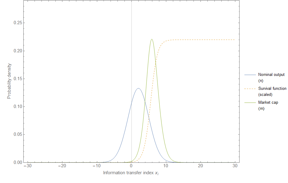
The market cap state distribution is in green with average ⟨m⟩ ~ 6 compared to the NGDP state distribution in blue with average ⟨n⟩ ~ 2. The latter is convolved with the logistic survival function (yellow dashed) to produce the former. Low index mᵢ firms are less likely to be listed. Although drawn from the same underlying distribution ⟨n⟩ ~ 2, survival bias represented by the survival function gives us ⟨m⟩ ~ 6 for the firms in the stock market

⁴

. In that sense the equity premium implies a diversified portfolio is safer than a random selection of investments (starting a restaurant, real estate speculation, collecting vintage Dougram toys, etc) in the economy at large.

This may or may not be true — it’s just a theoretical model using the information equilibrium framework that provides a way of looking at the equity premium puzzle. It’s interesting because the picture is not so much about agent behavior regarding risk, but rather the shapes of different opportunity sets. Agents in this model are just continuing to do their “so complex they seem random” thing of exploring the state space. The equity premium is more due to the differences in the institutions of the stock market versus government bonds and how they shape the state space agents operate within.

1. We are using the partition function approach for an ensemble of markets as described in my paper. Ensemble averages are indicated with angle brackets.

2. Side note: ⟨AD⟩ ~ Π AS, i.e. nominal output/aggregate demand is proportional to the price level times the amount of aggregate supply — as would be sensible.

3. The standard claim is something like 80% of new businesses fail in their first year, but seems that it’s more like 70% fail in 10 years, with 80% surviving their first year. Suffice to say, there is still a lot of churn.

4. For more on stocks and m-states, including how the distribution relates to alpha, beta, Tobin’s Q, etc see here (called them k-states at the link, but that’s because the information transfer index is k there).