Utility in an information equilibrium model

I've said many times on this blog that the concept of utility is unnecessary (except to solve an information problem); in this post I'll allow utility, but show that even then utility maximization is unnecessary to select an economic equilibrium.  Essentially, I will derive the utility approach to economics using the information transfer model.
Let's define utility $U(x_{1}, x_{2}, ...)$ to be the information source in the markets
$$
MU_{x_{i}} : U \rightarrow x_{i}
$$

for $i = 1 ... D$ where $MU_{x_{i}}$ is the marginal utility (a detector) for the good $x_{i}$ (information destination). We can immediately write down the main information transfer model equation:
$$
MU_{x_{i}} = \frac{\partial U}{\partial x_{i}} = k_{i} \; \frac{U}{x_{i}}
$$

Solving the differential equations, our utility function $U(x_{1}, x_{2}, ...)$ is
$$
U(x_{1}, x_{2}, ...) = a \prod_{i} \left( \frac{x_{i}}{c_{i}} \right)^{k_{i}}
$$

which is a Cobb-Douglas utility function ($a$ and the $c_{i}$ are constant). In the traditional economic approach, the next step is to look at the level curves of this utility function alongside the budget constraint (in a two-good market i.e. two dimensions):
$$
\text{(1) }\; M \geq \sum_{i} p_{i} x_{i} = p_{1} x_{1} + p_{2} x_{2}
$$

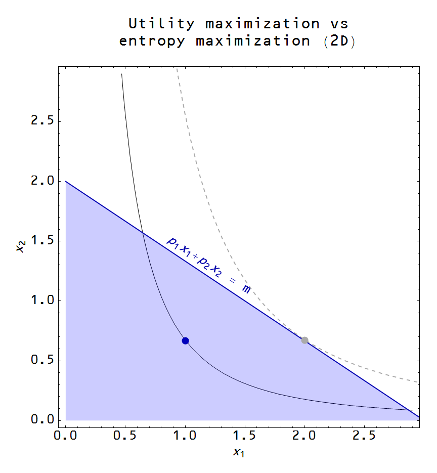
The level curve that is tangent to the budget constraint gives us the maximized utility. We show this in the next graph (level curve is the dashed gray curve and the maximized utility point is gray as well):

The entropy maximizing solution is given as the blue dot at the centroid of the blue triangle with the solid utility level curve passing through it. If we take every point that satisfies the budget constraint (1) as equally likely (the blue shaded region), the expected equilibrium value is given by the centroid. Now this centroid moves in effectively the same way as the utility maximum, just at a lower utility value:

The red line shows that at a higher price of $x_{1}$ with the same budget constraint, less of $x_{1}$ can be afforded. Both the utility maxima (gray dots) and the entropy maxima (blue and red dots) move inward towards smaller $x_{1}$ and lower utility, tracing out a demand curve. For two goods, there is only one big difference in the utility maximizing and entropy maximizing models of supply and demand: the entropy maximizing equilibrium doesn't fully saturate the budget constraint.

One possibility is to make the artificial restriction that all income $M$ must be spent. The centroid of the boundary of the blue triangle would essentially be the middle point of the budget constraint line. However, we don't actually have to do this.

If we randomly sample the triangle bounded by the budget constraint, we end up with something like this in two dimensions:

The distribution of the sum $p_{1} x_{1} + p_{2} x_{2}$ is somewhat uniformly distributed between 0 and the budget constraint as shown by the blue line in the next graph:

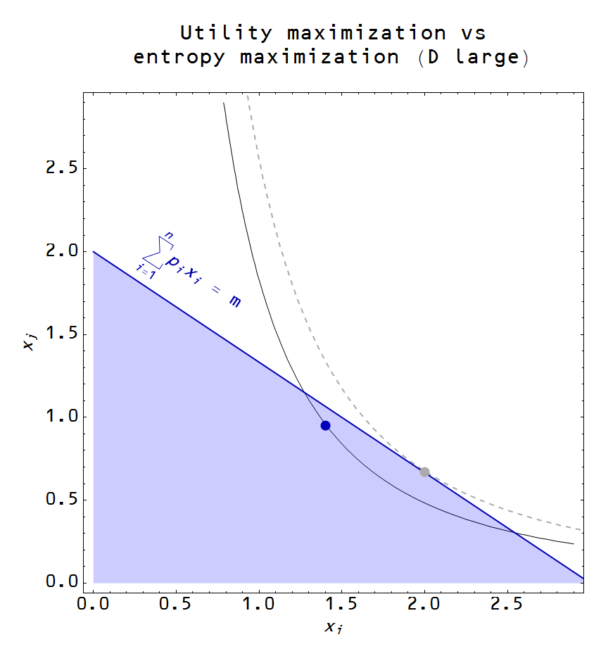
However, if we increase the number of dimensions (the number of goods in the economy), most of the points are near the budget constraint (the red and green lines). This is a general property of higher dimensional shapes: nearly all of the points are in a thin shell near the surface. That means for a large number of dimensions, the expected equilibrium should be near the budget constraint even without making the artificial restriction above:

Now this point only maximizes utility if every good is in a sense the same -- the budget constraint (1) and the utility function $U$ is symmetric under interchange of $x_{i} \leftrightarrow x_{j}$. Typically, the entropy maximizing point is near the utility maximizing point if neither the utility function nor the budget constraint are wildly asymmetric ($k_{i} \gg k_{j}$ or $p_{i} \gg p_{j}$).

We can't directly observe utility, though. Therefore it is always possible to perform a preference-preserving transformation $f(x_{i}, \alpha_{i}) : x_{i} \rightarrow \exp \alpha_{i} \log x_{i}$ that makes the utility level surface tangent at the maximum entropy point near the budget constraint (or makes the utility function symmetric). [Correction, per LAL in comments below.]

Aside: This framework would allow us to experimentally determine whether utility maximization or entropy maximization represented a better model of microeconomics. Using multiple goods, aggregate the different allocations chosen by individual subjects (every student in a classroom is given $n$ tokens to allocate among $m$ different goods like candy bars or bacon).

Second aside: The typical economics approach appears to be setting $MU_{x_{i}} = \beta p_{i}$; we could accommodate that with an additional information equilibrium condition $MU_{x_{i}} \sim p_{i}$ which would allow $\log MU \simeq k \log p$. The typical approach assumes $k = 1$.