The ISLM model (again)

The economist John Hicks wrote out Keynes' prose as an economic model that came to be known as the IS-LM model. I already derived this model before in a way that followed the way it is introduced in macroeconomics classes (as an IS and LM market). This derivation will acheive the same result, but approached fundamentally as an information transfer market system. The basis for the IS-LM model is that there are two markets: the real economy (IS) and the money market (LM) that couple to each other through the interest rate. As an information transfer system, we'll take a more direct route. We will posit that aggregate investment (demand) is a source of information that sends signals into the market that are detected by interest rate changes. The aggregate investment supply (the money supply) receives this information. See this post for a more detailed description of how information moves around the economy.
Let's start with the market $r : I \rightarrow M$, with interest rate $r$, nominal investment $I$ and money supply $M$ so that
$$
\text{(1) } r = \frac{dI}{dM} = \frac{1}{\kappa} \; \frac{I}{M}
$$

from the basic information transfer model. Looking at constant information source $I = I_{0}$, we have
$$
r =  \frac{1}{\kappa} \; \frac{I_{0}}{\langle M\rangle}
$$

where $\langle M \rangle$ is the expected level of the money supply.  Solving the differential equation (1), we obtain
$$
\Delta I \equiv I-I_{ref} = \frac{I_{0}}{\kappa}\log \frac{\langle M\rangle}{M_{ref}}
$$

where $ref$ refers to reference values of the variables $I$ and $M$. We can combine the previous two equations into a single function that defines the IS curve:
$$
\text{(2) }\log r = \log \frac{I_{0}}{\kappa M_{ref}} - \kappa \frac{\Delta I}{I_{0}}
$$

We can also look at constant $M = M_{0}$ so that we have, solving the differential equation (1) again:
$$
r =  \frac{1}{\kappa} \; \frac{\langle I\rangle}{M_{0}}
$$

$$
\Delta M \equiv M-M_{ref} = \kappa M_{0} \log \frac{\langle I\rangle}{I_{ref}}
$$

where we can eliminate $\langle I\rangle$ to produce (after some re-arranging)

$$
\text{(3) } \log r = - \log \frac{\kappa M_{0}}{I_{ref}} + \frac{\Delta M}{\kappa M_{0}}
$$

Equations (2) and (3) represent how the market adjusts the interest rate to changes in the money supply given fixed investment demand and to changes in the investment demand given fixed money supply, respectively.
One more piece -- we need to relate output $Y$ to investment $I$ and money $M$. I'll add a simple market $p : N \rightarrow I$ where $N$ is NGDP (aggregate demand, sending information to aggregate investment) so that
$$
\frac{dN}{dI} = \frac{1}{\eta} \; \frac{N}{I}
$$

which we solve without holding either constant, resulting in:

$$
N \sim I^{1/\eta}
$$

It turns out empirically (see below), $\eta \simeq 1$ so that $\log N$ is proportional to $\log I$. If we hold the price level constant (we are looking at short run effects [1]), then we can say that $Y = N/P$ is proportional to $I$. This is the first part. To get the relationship with $M$, we'll match first order shifts of the IS and LM curves. If we have a small change in $r = r_{0} + \delta r$, then we have for the IS curve:
$$
\log r_{0} + \frac{\delta r}{r_{0}} + \cdots = \log \frac{I_{0}}{\kappa M_{ref}} - \kappa \frac{\Delta I}{I_{0}}
$$

So that

$$
\frac{\delta r}{r_{0}} \simeq - \kappa\frac{\Delta I}{I_{0}}
$$

Similarly for the LM curve

$$
\frac{\delta r}{r_{0}} \simeq \frac{\Delta M}{\kappa M_{0}}
$$

So that we have (after taking the absolute value as a postitive shift of the LM curve causes the interest rate to fall, but a positive shift in the IS curve causes the interest rate to rise)
$$
\Delta I \simeq \frac{I_{0}}{\kappa^{2} M_{0}} \Delta M
$$

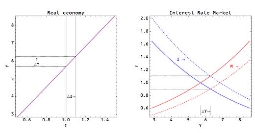
Which means $\Delta Y \sim \Delta I \sim \Delta M$ are all proportional to each other and we can scale the IS and LM curves such that they become functions of $Y$. This allows us to plot them on the same graph, like the ISLM model. On the left, we have the relationship between $I$ and $Y$ and on the right, we have the IS-LM model graph (IS curve in blue, LM curve in red):

Empirically, it works best if we take $r \rightarrow r^{c}$ where $c \simeq 1/3$ [2] ($M$ is taken to be the monetary base):

And as promised, here is that plot of investment vs NGDP:

[1] This is effectively where economists' complaint about the IS-LM model not incorporating inflation (by not differentiating real and nominal interest rates) comes in.
[2] This is a fudge that I have yet to figure out. The empirical results for the 10-year and 3-month interest rates are a pretty good motivation. It fits the data. Additionally, it is basically a re-labeling of the interest rates. There is no a priori reason that the "information price" $p_{i}$ that goes into Equation (1) and the real world price represented by the interest rate $r$ need to be related by $r = p_{i}$; any bijective relationship is possible. We encounter this all the time e.g. decibels give us a more intuitive linear feeling of loudness than power. The market treats the cube root of the interest rate as a linear measure of information.

UPDATE 5/22/2015

Fixed the fudge factor. See here. Basically introduced another information equilibrium relationship between $r$ and the price of money $p$ so that the market at the top of the page becomes:
$$
(r \rightarrow p) : I \rightarrow M
$$

And therefore $r \sim p^{1/c}$