The IS-LM model as an effective theory at low inflation
No one seems to like the poor old IS-LM model except Paul Krugman. I thought I'd defend it as an effective macro theory. What does that mean? It means it is a theory that operates given a certain scope. For IS-LM, assuming the IT model is the "true" theory, that scope is low inflation. Here's how it works:
Start with the AD-AS model (with aggregate demand aka nominal output N and aggregate supply S), and introduce money (M)
N ⇄ S
N ⇄ M ⇄ S
The produces an information equilibrium relationship
P : N ⇄ M
The P just names the abstract price (the price level) and the above notation means:
P ≡ dN/dM = k (N/M)
We can solve this differential equation to obtain:
N ~ Mᵏ
P ~ k Mᵏ⁻¹
That should be a k - 1 in the exponent, not (M^k)^-1. If k ≈ 2, then we have P ~ M (a "quantity theory of money" where inflation is money growth). If k ≈ 1 (one way of stating our scope condition), then
N ~ M
P ~ constant
so that inflation π ≈ 0 (another way of stating our scope condition [1]). If inflation is "small", then
N ~ Y
where Y is real output. Now let's introduce another set of information equilibrium relationships
p : N ⇄ MB
i ⇄ p
where MB is the monetary base, p is the abstract price of money and i is the nominal (short term) interest rate. If π ≈ 0, then we can write this as:
p : Y ⇄ MB
r ⇄ p
using N ~ Y and i ~ r where r is the real interest rate. The differential equations associated with this pair of information equilibrium relationships has a similar solution in general equilibrium to the one above, but I'll write it differently:
(1) log(r) = c log(b Y/MB)
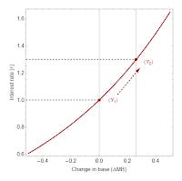
Now which variables do you think will react the fastest to monetary expansion? I'd go with the monetary base and the interest rate, rather than real output. That puts us on the partial equilibrium solution where Y "moves last" (in economics parlance). In physics terms, this is analogous to an isothermal expansion of an ideal gas (an 'iso-output' expansion of an economy) that looks like this:


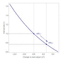
Those angle brackets mean ensemble averages (weighted average over random markets).
The interest rate falls and the monetary base expands from MB₁ to MB₂. Note at this level of effective theory, it is not important which one causes the other one -- increasing the base lowers interest rates or lowering interest rates expands the base. As Y rises, interest rates will come back up and equation (1) will hold -- general equilibrium restored.
What about fiscal policy? That's the second diagram above. In that case, the central bank "moves last". Fiscal expansion should take us from Y₁ to Y₂, but if the central bank didn't let rates rise or the base expand, you could end up back where you started. This is the basic monetary offset picture that happens when inflation is low and nominal (and real) interest rates are positive.
That captures most of the mechanics of the IS-LM model; you could rewrite this in terms of investment if you wanted (as I do here). And there is a bit more to the details of how it works, but the theories are roughly isomorphic to each other.
Paul Krugman points out in the liquidity trap argument everything changes at the zero lower bound (or basically, anytime interest rates are very low ... remember we're still in a limit where inflation is very low as well). This is the limit where r ≈ 0⁺. Here we have a different-looking pair of diagrams:


The general idea is the same, but the magnitudes are very different. A large expansion of the base drops your interest rate to zero without moving output very far to the right (monetary expansion is ineffective). A large fiscal expansion can happen without large movement in the monetary base (i.e. monetary offset doesn't work). In this case, we have a model that captures the essence of the liquidity trap.
Recall that we built this out of the AD-AS model, but we did it by restricting the scope to r ≈ 0⁺, π ≈ 0 (or just π ≈ 0 for the IS-LM model) [1]. This doesn't mean this model is right, but it does mean if you are using the AD-AS model where inflation is low and interest rates are low, then you are effectively using the IS-LM model (if you are doing it correctly).
And since the above model does pretty well empirically (see the paper or the forecasts), it means that any theory that describes the data (when π ≈ 0) will also be approximated by the IS-LM model.
An analogy: since Newton's inverse square law describes the orbits of planets fairly well, any theory that describes the orbits of planets fairly well will be approximated by Newton's inverse square law. This is actually true of general relativity (which reduces to Newton's inverse square law) and will also be true of the fundamental quantum theory of gravity -- should it exist.
...
Footnotes
[1] Strictly speaking, these inflation and interest rates are small compared to some other scale in the theory, in this case we could use the average growth rate of the monetary base (minus reserves) r << μ, π << μ. In the US, this has been about 7% per year. Inflation is about 1-1.5% and (short term, nominal) interest rates are 0.3-0.5% -- both are less than 7% and that gives us an idea that the error in this model could be ~10% ... i.e. 0.005/0.07 ~ 0.01/0.07 ~ 0.1.


