The Economy at the End of the Universe, part II

Nick Rowe asked in a comment on this post if I could look at the second model (a Cagan monetary demand model) he describes in his post and that took me on an adventure that might be enlightening. I also thought about calling this post Life, the Universe and Economics (or something like that) as the sequel to the previous post.
Anyway, a Cagan model has $M/P$ (real money supply) as a negative function of expected inflation, so using rational expectations (model-consistent expectations) and taking $\log M \equiv m$ and $\log P \equiv p$ we have
$$
\log M/P = m - p = - \tau \pi^{E} = - \tau \frac{d}{dt} \log P = - \tau \dot{p}
$$

The general (forward-looking) solution to this equation is an integral of the money supply (or monetary base or what have you)
$$
p(t) = \frac{1}{\tau} \int_{t}^{\infty} dt' e^{\frac{t-t'}{\tau}} m(t')
$$

As an aside, this is an example of using a Laplace transform to solve a differential equation. We can see that $\tau$ is essentially a time horizon. It weights the future (expected) money supply by a decreasing exponential factor (similar to a discount factor).
But that infinity is also a time horizon -- it tells us where to stop considering the future at all. Note that times $T \gg \tau > t$ don't contribute much to the integral. If we look at the limiting behavior of this integral (at times $t$ in the distant future after any impact of a shock to monetary policy such that $m(t) = \mu t$ -- constant money growth) we have:
$$
P(t) = \exp \; p(t) = \exp \; \left( \mu (t + \tau) - e^{(t-T)/\tau} (T + \tau) \right)
$$

This has two different limits depending on whether you take $\tau$ to infinity first (it's 0) or $T$ to infinity first (it's infinite). Again, we have the same issue as we had with Nick Rowe's reductio ad absurdum and the conclusion we should draw is that only the limits $T \gg \tau$ and $\tau \gg T$ could make sense. There's either rapid discounting or slow discounting (those limits just mentioned, respectively) at the horizon. And in those two cases we have either $P \sim \exp \mu t$ (steady growth in the price level) or $P \sim 1$ (i.e. constant, but with a growing money supply).
If we take the first limit we have something that looks basically like the previous post (except the steady state has constant growth, which we could have chosen for the previous model but didn't for simplicity):

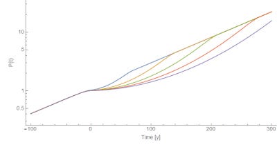
In any case, we have the same problem that as the time horizon $t_{0}$ at which $m(t_{0})$ returns to "normal" moves out, the result differs by a larger and larger amount from $P \sim \exp \mu t$. Here's the graph of inflation ($\dot{p}(t)$):

Note that the Cagan model has different results [pdf] for adaptive expectations. Depending on parameters, inflation is either basically monetary (it depends on $m(t)$ Nick Rowe's concrete steppes) or basically expectations (i.e. is independent of $m(t)$). The former limit is either rapid discounting, rapid adaptation, or both. The latter is either slow discounting, slow adaptation. or both (but results in exploding inflation).

...

Addendum

It is interesting to look at this model as an information transfer model $X : M \rightleftarrows P$ where "expectations" $X$ are the detector of information equilibrium between the money supply and the price level
$$
k \frac{M}{P} = \frac{dM}{dP} \equiv X = e^{-\tau \pi^{E}}
$$

Or in the form above, using $x = \log X$

$$
m - p + \log k = x
$$

In general equilibrium we have

$$
X \sim P^{k -1}
$$

so if we use rational expectations, we must equate the price $X$ with the value of $X$ above such that
$$
X \sim e^{(k-1) \log P} \sim e^{- \tau \pi^{E}} \equiv e^{-\tau \frac{d}{dt} \log P}
$$

and we discover the operator formula

$$
-\tau \frac{d}{dt} = k - 1
$$

when acting on $p = \log P$. That means

$$
P \sim \exp \left( \exp \left( \frac{1-k}{\tau} t \right) \right)
$$

That's not a typo -- it's a double exponential. In order to have $P$ not explode (given rational expectations), we need $k = 1$, which implies that the price level is constant. This is exactly the same finding as a more traditional approach to the Cagan model [pdf].  The resolution here depends on what model you trust more. If you trust rational expectations, then you question the equilibrium. If you trust information equilibrium, you question rational expectations.
...
PS Gosh, I had to think about this for nearly two weeks and over three flights. I may still have gotten it wrong. Weird and subtle things can happen when you have to deal with infinity.
PPS You can see the limits pretty directly just looking at the equation
$$
m - p = - \tau \dot{p}
$$
If $\tau \gg T$, then you have $- \tau \dot{p} \approx 0$, and thus $P \sim 1$. If $T \gg \tau$, then you have $m - p \approx 0$ and so $P \sim M(t) \sim \exp \; \mu t$ in my example.